Gr/Ni(111) Registry and Work of Adhesion

1. Introduction

This tutorial reproduces the structure and energetics of graphene on Ni(111) — which registry the film adopts, how far it sits above the surface, and the work of adhesion of each arrangement — using the interface created in the structure creation tutorial.

Manuscript

Arjun Dahal, Matthias Batzill, "Graphene-nickel interfaces: a review" Nanoscale, 6(5), 2548 (2014) DOI: 10.1039/c3nr05279f ¹

1.1. What is being reproduced

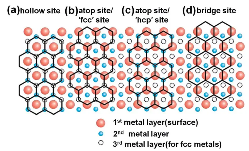
Graphene and Ni(111) are lattice-matched to within a fraction of a percent, so the film locks into a 1×1 registry. The review's section 2.1 collects the established structural facts: LEED I–V and ion scattering identify the adsorbed structure as one carbon atop a first-layer Ni atom and the other in the fcc hollow, 0.211 nm above the surface, with a 0.005 nm buckling in which the atop carbon sits further out. The review's computed values come from Lahiri et al., New J. Phys. 13, 025001 (2011) — open access, and the quantitative target here (its Table 1):

interface	work of adhesion (J/m²)	separation (Å)
fcc (atop + fcc hollow)	0.81	2.16
hcp (atop + hcp hollow)	0.77	2.17
hollow (fcc + hcp hollows)	0.31	3.26

The review's text quotes the hollow as 0.38 J/m²; the source paper's Table 1 says 0.31, and the notebook targets the source. The bridge registry (Fig. 1d of the review) is not quantified in either paper and is computed as an extra point beyond the published set.

1.2. The published recipe, and why relaxation is not optional

Lahiri et al. state their method plainly: LDA, because "GGA does not provide an adequate description of Ni–graphene bonding" for this interface; spin-polarized throughout; and geometry relaxation with the bottom substrate layers fixed. The buckling is itself one of the published numbers, and no rigid placement can produce a buckling — so every result in this tutorial comes from a relaxed structure, and rigid scans are used only to bracket the starting separations.

2. Prerequisites

Run the structure creation tutorial first. Its notebook builds the Gr/Ni(111) interface and saves it into the uploads folder as Graphene_Nickel_interface; the simulation notebook loads it back by exactly that name and stops if it is missing. The reduced cell is the 1×1 match: 2 carbon and 4 nickel atoms.

3. What is calculated

Two tiers, both relaxed:

1. Fast tier — MACE-MP + D3, in the browser. Each registry is placed (the surface sites are measured from the substrate's own top layers, and each registry label is re-verified after relaxation, so a structure that slid into a neighbouring registry cannot be reported under the wrong name), bracketed by a rigid scan, then relaxed with the bottom substrate layers fixed — the paper's scheme. Same-cell relaxed references (bare Ni slab, free-standing graphene) turn the energies into works of adhesion: W = [E(slab) + E(graphene) − E(interface)] / A.

The fast tier is expected to fail the energetic targets, and says so. MACE-MP is PBE-trained, and PBE-level physics is exactly what the paper rejects for this interface: chemisorption comes out several times too weak. What the fast tier is good for is the geometry survey — the E(z) curves, the two-minimum structure, and the dispersion-bound hollow, whose work of adhesion it nearly matches (0.30 vs 0.31 J/m²). Its comparison table prints against the paper's values with pass/fail per check and an honest per-tier verdict line.

1. Precise tier — the paper's LDA on the platform. One relaxation + total-energy job per selected registry, starting from the MACE-relaxed geometry, plus the two same-cell references — LDA (pz, GBRV ultrasoft — the platform carries the LDA set for both Ni and C), spin-polarized, no dispersion correction, matching the paper: LDA binds this interface unaided, which is the stated reason its authors chose it. This tier carries the reproduction claim.

registry	Fig. 1	carbon sublattices	published target
atop_fcc	(b)	atop + fcc hollow	0.81 J/m² at 2.16 Å, favourable
atop_hcp	(c)	atop + hcp hollow	0.77 J/m² at 2.17 Å
hollow	(a)	fcc + hcp hollows	0.31 J/m² at 3.26 Å — dispersion-bound
bridge	(d)	C–C bond straddling a first-layer Ni	beyond the published set

4. Calculation parameters

	fast tier	precise tier	Lahiri et al.
Method	MACE-MP-0 (large, float64) + D3	LDA (pz), GBRV ultrasoft	LDA, all-electron LCAO (DMol)
Spin	via training data	collinear, moment started at 0.7 μB on Ni	spin-polarized (bulk Ni: 0.56 μB)
Relaxation	BFGS, bottom 2 Ni layers fixed	platform relaxation + total energy	bottom 2 of 5 Ni layers fixed
Cutoffs	—	40 / 200 Ry (GBRV's published pair)	all-electron
k-grid	—	12×12×1 (multiple of 3, so K is on the mesh)	converged, not stated
Smearing	—	Marzari-Vanderbilt cold, degauss = 0.01 Ry	not stated
Dispersion	D3	none — matching the paper	none

Stated divergences from the paper: the slab is the structure tutorial's 4 Ni layers rather than 5; the vacuum is 20 Å rather than 90; the platform relaxation cannot hold the bottom layers fixed (the fast tier can, and does); plane-wave pseudopotentials rather than all-electron LCAO. The SCF convergence settings (cold smearing, local-TF mixing, mixing_beta = 0.2, 200 iterations) exist because the platform defaults stop at "convergence NOT achieved after 100 iterations" on this spin-polarized metal slab, with the energy oscillating in its fourth decimal — charge sloshing.

5. Step-by-step instructions

5.1. Create the structure

Run the structure creation notebook. It saves Graphene_Nickel_interface into uploads.

5.2. Open the simulation notebook

other/materials_designer/specific_examples/optimization_interface_film_xy_position_graphene_nickel_SIMULATION.ipynb

5.3. Run the fast tier

Run > Run All Cells. Sections 2–4 need no platform account: they load the interface, derive and verify the registries, relax each one with MACE, and print the comparison against Lahiri Table 1 — including the honest [MACE tier] verdict.

5.4. Run the precise tier

Section 5 authenticates and submits, per selected registry, a relaxation + total-energy job at the paper's LDA, plus the two reference jobs. A default run selects one registry — three jobs. Leaving DFT_REGISTRY_NAMES empty skips the platform tier entirely; the automated test does exactly that, because relaxation jobs outlast what a browser test may wait for.

5.5. Read the verdict

The final cell restates the published targets and prints one verdict per tier:

Reproduces Lahiri et al. Table 1 [MACE tier]: no
Reproduces Lahiri et al. Table 1 [DFT tier]: yes

The fast tier failing its energetic checks is the physics working as documented, not a bug — see section 3. The DFT-tier line appears once the selected registries and both references have finished.

6. Troubleshooting

If a registry's rigid scan finds no bracketed minimum, widen the scan window. If every registry comes back physisorbed-only in the fast tier, check MACE_MODEL and MACE_DEFAULT_DTYPE — the medium/float32 combination misses the chemisorbed minimum entirely. The first MACE call downloads the foundation model; later runs use the cache. If a platform job stops at "convergence NOT achieved", the smearing/mixing block in the parameters cell is the knob — those settings exist precisely because the defaults do not converge this slab.

7. Interactive JupyterLite notebook

The notebook below runs the fast tier and, when registries are selected, the platform tier. Select Run > Run All Cells.

⛶ Full Screen

8. References

---

1. Arjun Dahal and Matthias Batzill. Graphene–nickel interfaces: a review. Nanoscale, 6:2548–2562, 2014. URL: https://doi.org/10.1039/C3NR05279F. ↩